Advanced SRT & Microphone Audio Visualization and Recording

---

Advanced SRT & Microphone Audio Visualization and Recording

This project provides an efficient, extensible Python script for:

1. Streaming audio via SRT (Secure Reliable Transport).
2. Recording microphone or SRT audio to a WAV file.
3. Visualizing audio data in real-time (waveform, FFT, and spectrogram) with Matplotlib.
4. Playing live streamed audio through speakers.

The code is designed to handle various modes (record-only, visualize-only, and full playback) with minimal user intervention, while keeping performance in mind for continuous data streams.

---

Table of Contents

• Overview
• Project Context
• Key Features
• Architecture
• Usage
• Final Visualization Example
• Performance Considerations

---

Overview

The goal of this project is to offer a flexible yet highly efficient way of handling audio input from both a local microphone and remote SRT streams. The script allows users to:

• Connect to a remote SRT address, capture incoming audio, and optionally record or visualize it.
• Use a local microphone for real-time capturing, either to record or to visualize, or both.
• Maintain a lightweight, fast main loop to minimize delays and lags.

Core Python libraries used include:

• sounddevice for local microphone streaming
• pyaudio for playback
• wave for WAV file I/O
• matplotlib for real-time plotting
• [queue, threading, subprocess] from the standard library for concurrency and SRT streaming via FFmpeg

---

Project Context

This project extends beyond simple audio visualization and playback, finding real-world applications in environmental monitoring and data analysis. For example:

• Marine Ecosystems: This tool has been successfully deployed in projects such as the Remote Monitoring of Coral Reef Underwater Sounds. In this context, SRT streaming is used to transmit underwater acoustic data from hydrophones in marine habitats, enabling researchers to monitor ecological health in real time.
• Signal Processing Research: The modular design of this application allows it to be adapted for various signal processing tasks, including real-time acoustic analysis, machine learning integration, and environmental sound classification.

Remote Monitoring of Coral Reef Underwater Sounds

Figure 1: A presentation poster highlighting the use of this tool for remote monitoring of underwater environments. (Note: May appear as a downloadable link depending on hosting platform.)

---

Key Features

1. Multiple Audio Sources
   • Microphone: Streams live audio from the system’s default recording device.
   • SRT: Connects to a remote SRT server using FFmpeg, handling packet buffering, jitter, etc.
2. Multiple Operation Modes
   • Record Only: Saves raw audio (16-bit PCM) to a WAV file without visualizing or playing it.
   • Visualize Only: Displays live waveform, FFT, and/or spectrogram with no file I/O.
   • Record + Visualize + Playback: Combines all features, letting users see, hear, and record simultaneously.
3. Robust Real-Time Visualization
   • Waveform: Displays the amplitude vs. time graph.
   • FFT Plot: Shows frequency components in near real-time.
   • Spectrogram: Visualizes frequency intensity over a rolling time window.
4. Flexible Configuration
   • Sample Rate: Dynamically determined or set for consistent FFT sizing.
   • FFT Window Size: Chosen to achieve a balance between frequency resolution and real-time responsiveness.
   • Frequency and Time Window: User can specify the range for FFT or spectrogram (e.g., 0–20 kHz).
5. Optimized Performance
   • Uses separate threads for audio reading, writing, and visualization to reduce blocking.
   • Employs a minimal logic loop for reading SRT or mic data, offloading visualization and file I/O to queues and threads where possible.

---

Architecture

The project’s architecture follows a streamlined and efficient pipeline for processing audio data in real time:

1. Audio Source
   Audio data is sourced either from:
   • Microphone: Captured using the system’s default recording device.
   • SRT Stream: Captured via FFmpeg, ensuring reliable packet delivery and minimal latency.
2. Main Loop
   The main loop performs minimal processing to avoid delays, delegating tasks to separate threads for:
   • Audio Callbacks: Capturing and queuing raw audio data.
   • Visualization Updates: Rendering waveform, FFT, and spectrogram plots.
3. Data Enqueuing
   Audio data is organized into separate queues for efficient, non-blocking operations:
   • raw_audio_queue: Stores raw PCM audio samples.
   • fft_queue: Stores frequency-domain data for FFT plots.
   • spectrogram_queue: Maintains rolling frequency-intensity data for spectrogram rendering.
4. Parallel Processing
   • Recording Thread: Writes audio data to a WAV file asynchronously.
   • Visualization Loop: Updates plots in real time using Matplotlib without interrupting audio acquisition.
5. Output
   The processed data is presented in two forms:
   • Visual Outputs: Waveform, FFT, and spectrogram plots displayed interactively.
   • Audio Files: Recorded audio saved as high-quality WAV files.

The architecture ensures a balance between high performance and real-time responsiveness, making it suitable for continuous audio streams.

---

Usage

Step 1: Interactive CLI Configuration

The application features an intuitive CLI that guides users through configuration:

• Source Selection: Choose between local microphone or SRT stream.
• Operation Mode: Record only, visualize only, or combined modes.
• Visualization Options: Enable Waveform, FFT, and/or Spectrogram.
• Time and Frequency Windows: Set parameters for visualization.

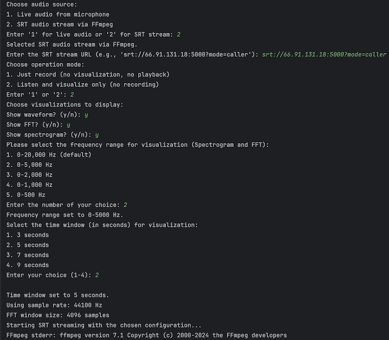
Figure 2: CLI prompts for configuring the application. Users select SRT streaming, choose “visualize only,” and configure specific plots, time, and frequency settings.

Step 2: Running the Application

Once configured:

• For microphone input, the audio stream begins instantly.
• For SRT streams, FFmpeg handles packet buffering, ensuring reliable data reception.

• Visualizations dynamically update as the audio data is processed.

Final Visualization Example

The following visualizations are generated in real time:

• Waveform: Shows amplitude vs. time.
• FFT Plot: Displays amplitude vs. frequency.
• Spectrogram: Illustrates intensity variations across frequencies over time.

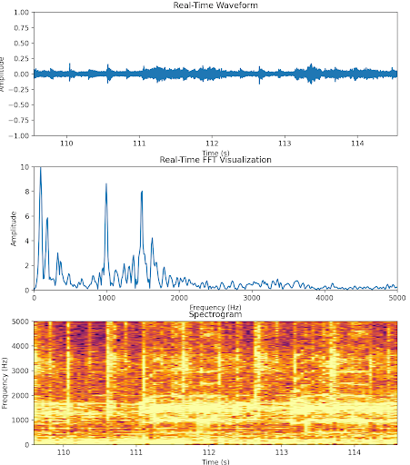
Figure 3: Real-time visualizations of waveform (top), FFT plot (middle), and spectrogram (bottom), providing comprehensive insights into the incoming audio stream.

---

Performance Considerations

• Threaded Approach: Decouples audio acquisition, file I/O, and visualization tasks to minimize bottlenecks.
• Asynchronous Visualization: Uses Matplotlib’s interactive mode for non-blocking updates, ensuring a smooth user experience.
• Dynamic Resource Management: FFT window size and queue processing are optimized for responsiveness.
• Minimal Callback Overhead: Audio callbacks are streamlined to enqueue data, leaving intensive tasks to background threads.

---